After reading this topic Peak overshoot $({M_p})$ in Time response of a second-order control system for subjected to a unit step input underdamped case, you will understand the theory, expression, plot, and derivation.
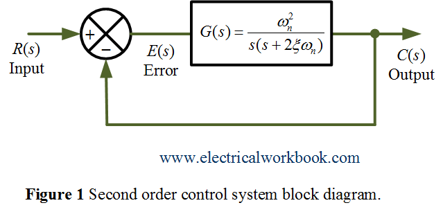
A block diagram of the second order closed-loop control system with unity negative feedback is shown below in Figure 1,
The general expression for the time response of a second order control system or underdamped case is
\[c(t) = 1 – \frac{{{e^{ – \xi {\omega _n}t}}}}{{\sqrt {1 – {\xi ^2}} }}\sin \left[ {({\omega _n}\sqrt {1 – {\xi ^2}} )t + \theta } \right]…(1)\]
Also Equation 1, is plotted in Figure 2 as shown below
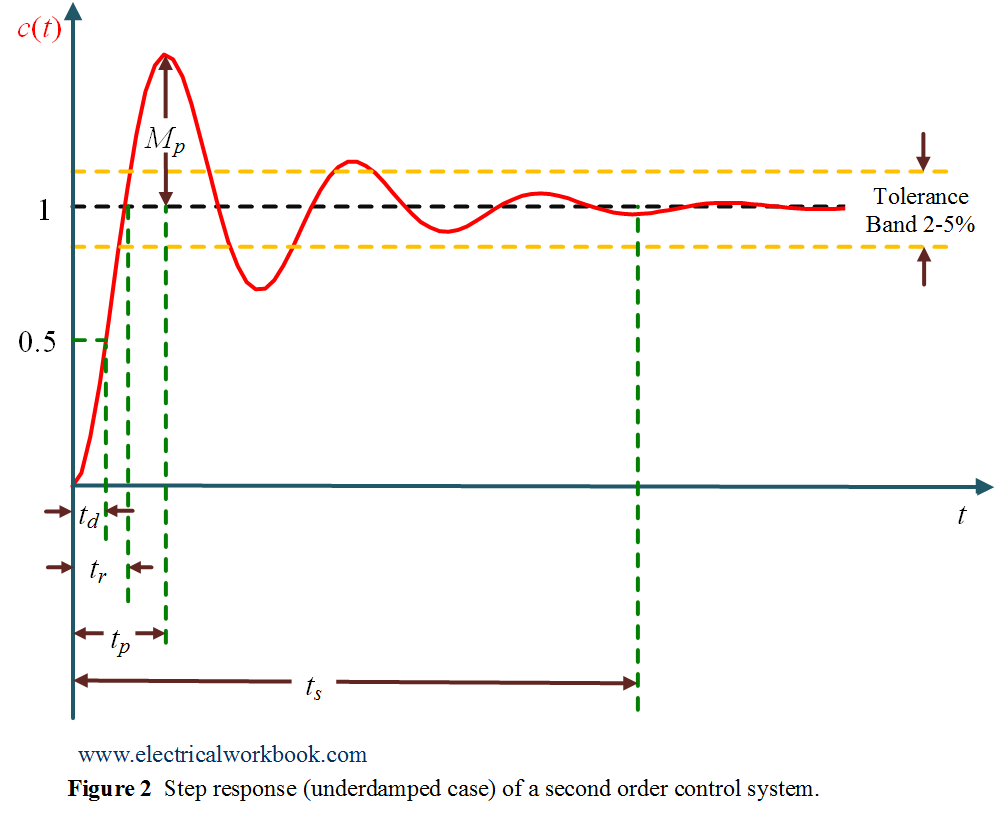
Peak overshoot $(M_p)$
It is the difference between first peak of overshoot for output and the steady state output value, i.e.
\[{\text{Peak overshoot (}}{M_p}) = c({t_p}) – c(\infty )\]
where, $c({t_p})$ is the first peak of overshoot for output $c(t)$ and $c(\infty )$ is the steady state output value of $c(t)$.
Also,
\[{\text{Peak percent overshoot (}}{M_p}){\text{ = }}\frac{{c({t_p}) – c(\infty )}}{{c(\infty )}} \times 100% \]
In second order underdamped system with unity step input, the steady state output $c(\infty )$ is unity, therefore
\[{M_p} = c({t_p}) – 1….(2)\]
\[% {M_p} = \frac{{c({t_p}) – 1}}{1} \times 100\]
Also, Equation 1 at time $t = {t_p}$ can be written as,
\[c({t_p}) = 1 – \frac{{{e^{ – \xi {\omega _n}{t_p}}}}}{{\sqrt {1 – {\xi ^2}} }}\sin ({\omega _d}{t_p} + \theta )….(3)\]
Using Equation 2 and Equation 3 gives
\[{M_p} = 1 – \frac{{{e^{ – \xi {\omega _n}{t_p}}}}}{{\sqrt {1 – {\xi ^2}} }}\sin ({\omega _d}{t_p} + \theta ) – 1\]
\[{M_p} = \frac{{{e^{ – \xi {\omega _n}{t_p}}}}}{{\sqrt {1 – {\xi ^2}} }}\sin ({\omega _d}{t_p} + \theta )….(4)\]
As first peak of overshoot for output value of $c(t)$ i.e. n = 1 using in general equation of peak time $({t_p})$ gives
\[{t_p} = \frac{{1.\pi }}{{{\omega _d}}}….(5)\]
Put Equation 5 in Equation 4 gives
\[{M_p} = \frac{{{e^{ – \xi {\omega _n}.(\pi /{\omega _d})}}}}{{\sqrt {1 – {\xi ^2}} }}\sin ({\omega _d}.\frac{\pi }{{{\omega _d}}} + \theta )\]
or,
\[{M_p} = \frac{{{e^{ – \xi {\omega _n}.(\pi /{\omega _d})}}}}{{\sqrt {1 – {\xi ^2}} }}\sin (\pi + \theta )….(6)\]
Put ${\omega _d} = {\omega _n}\sqrt {1 – {\xi ^2}} $ in Equation 6 gives
\[{M_p} = \frac{{{e^{ – \xi {\omega _n}.(\pi /({\omega _n}\sqrt {1 – {\xi ^2}} ))}}}}{{\sqrt {1 – {\xi ^2}} }}\sin (\pi + \theta )\]
or simply,
\[{M_p} = \frac{{{e^{ – \xi \pi /(\sqrt {1 – {\xi ^2}} )}}}}{{\sqrt {1 – {\xi ^2}} }}\sin \theta ….(7)\]
Since,
\[\sin \theta = \sqrt {1 – {{\cos }^2}\theta } = \sqrt {1 – {\xi ^2}} ….(8)\]
Using Equation 7 and Equation 8 gives
\[{M_p} = \frac{{{e^{ – \xi \pi /(\sqrt {1 – {\xi ^2}} )}}}}{{\sqrt {1 – {\xi ^2}} }}\sqrt {1 – {\xi ^2}} \]
or simply,
\[{M_p} = {e^{ – \xi \pi /(\sqrt {1 – {\xi ^2}} )}}\]
Also, Peak percent overshoot will be
\[% {M_p} = \frac{{{e^{ – \xi \pi /(\sqrt {1 – {\xi ^2}} )}}}}{1} \times 100\]
or simply,
\[% {M_p} = {e^{ – \xi \pi /(\sqrt {1 – {\xi ^2}} )}} \times 100\]