After reading this topic Second order control system, you will understand the open and close loop transfer function, characteristic equation, Pole – zero map (undamped, underdamped and overdamped), root locus, example, and block diagram.
In a system whose transfer function having the highest power of s equal to 2 in its denominator, is called the second order control system.
Closed-loop transfer function and block diagram
A block diagram of the second order closed-loop control system with unity negative feedback is shown below in Figure 1,
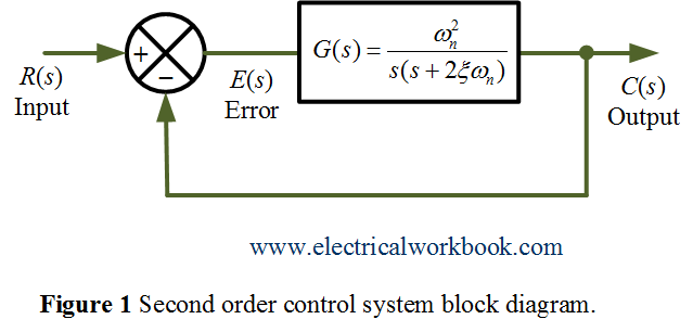
Here, ${\omega _n}$ is the undamped natural frequency in rad/sec and $\xi$ (geta) is the damping ratio.
So, the open loop transfer function of second order control system can be written as
\[G(s) = \frac{{\omega _n^2}}{{s\left( {s + 2\xi {\omega _n}} \right)}}\]
also given unity negative feedback,
\[H(s) = 1\]
The close loop transfer function of second order control system can be written as
\[\frac{{C(s)}}{{R(s)}} = \frac{{G(s)}}{{1 + G(s)H(s)}} = \frac{{\omega _n^2/[s(s + 2\xi {\omega _n})]}}{{1 + \omega _n^2/[s(s + 2\xi {\omega _n})]}}\]
\[\frac{{C(s)}}{{R(s)}} = \frac{{\omega _n^2}}{{{s^2} + 2\xi {\omega _n}s + \omega _n^2}}….(1)\]
Equation(1) is the standard form or transfer function of second order control system and equating its denominator to zero gives,
\[{s^2} + 2\xi {\omega _n}s + \omega _n^2 = 0….(2)\]
Equation(2) called the characteristic equation of second order control system. The roots of characteristic equation are the closed loop poles of the second order control system. Equation(2) is in the form of quadratic equation and hence roots will be
\[{s_1},{s_2} = \frac{{ – 2\xi {\omega _n} \pm \sqrt {{{\left( {2\xi {\omega _n}} \right)}^2} – 4\omega _n^2} }}{2}\]
\[ = – \xi {\omega _n} \pm {\omega _n}\sqrt {{\xi ^2} – 1} \]
\[ = – \xi {\omega _n} \pm j{\omega _d}….(3)\]
where imaginary part ${\omega _d}$ is the damped frequency in rad/sec.
Pole-zero map
Using Equation 3, the Pole-zero map of a second-order system is shown below in Figure 2. Equation 3 depends on the damping ratio $\xi$, the root locus or pole-zero map of a second order control system is the semicircular path with radius $\omega _n$, obtained by varying the damping ratio as shown below in Figure 2.
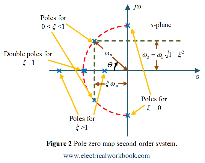
In Figure 2, for $\xi$ = 0 is the undamped case, for $\xi$ = 0 is the undamped case, for $\xi$ = 0 is the undamped case, and for $\xi$ = 0 is the undamped case
Examples
All analog indicating instruments (like PMMC), series RLC network.
Consider the series RLC network which is an example of a second order system, as shown below in Figure 3.
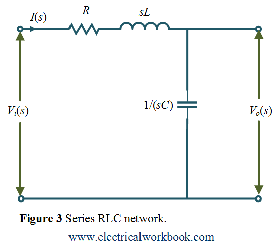
Using KVL, the input voltage ${V_i}(s)$ across series RLC network can be written as
\[{V_i}(s) = I(s)\left( {R + sL + \frac{1}{{sC}}} \right)\]
\[ = I(s)\left( {\frac{{1 + sCR + {s^2}LC}}{{sC}}} \right)\]
The output voltage ${V_o}(s)$ across capacitor can be written as
\[{V_o}(s) = I(s)\left( {\frac{1}{{sC}}} \right)\]
The ratio of output voltage ${V_o}(s)$ to the input voltage ${V_i}(s)$ can be written as
\[\frac{{{V_o}(s)}}{{{V_i}(s)}} = \frac{1}{{1 + sCR + {s^2}LC}}\]
\[\frac{{{V_o}(s)}}{{{V_i}(s)}} = \frac{{(1/LC)}}{{{s^2} + (R/L)s + (1/LC)}}…..(3)\]
By comparing Equation 3 with Equation 1 (the second order control system standard form) as
\[{s^2} + 2\xi {\omega _n}s + \omega _n^2 = {s^2} + \frac{R}{L}s + \frac{1}{{LC}}\]
which gives
\[\omega _n^2 = \frac{1}{{LC}}\]
or,
\[{\omega _n} = \frac{1}{{\sqrt {LC} }}\]
also,
\[2\xi {\omega _n} = \frac{R}{L}\]
\[\xi = \frac{R}{2}\sqrt {\frac{L}{C}} \]