After reading this topic Time response of a second-order control system for underdamped case subjected to a unit step input, you will understand the theory, expression, plot, and derivation.
In a system whose transfer function having the highest power of s equal to 2 in its denominator, is called the second order control system.
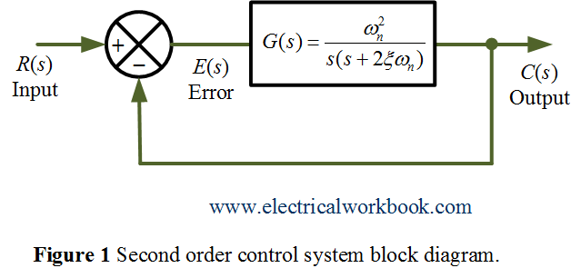
Closed-loop transfer function and block diagram
A block diagram of the second order closed-loop control system with unity negative feedback is shown below in Figure 1,
For underdamped case, the step-response of a second-order is
\[C(s) = R(s)\frac{{\omega _n^2}}{{{s^2} + 2\xi {\omega _n}s + \omega _n^2}}…(1)\]
The input to the system is unit step function, so in s-domain,
\[R(s) = \frac{1}{s}……(2)\]
and in time (t) domain, input unit step function is
\[r(t) = 1\]
Using Equation 1 and Equation 2 gives,
\[C(s) = \frac{1}{s}.\frac{{\omega _n^2}}{{{s^2} + 2\xi {\omega _n}s + \omega _n^2}}….(3)\]
Applying partial fraction on Equation 3 gives
\[C(s) = \frac{1}{s} – \frac{{s + 2\xi {\omega _n}}}{{{s^2} + 2\xi {\omega _n}s + \omega _n^2}}……(4)\]
The denominator term ${s^2} + 2\xi {\omega _n}s + \omega _n^2$ of Equation 4 can be written as
\[{s^2} + 2\xi {\omega _n}s + \omega _n^2 = {(s + \xi {\omega _n})^2} + \omega _n^2(1 – {\xi ^2})….(5)\]
Also,
\[\omega _d^2 = \omega _n^2(1 – {\xi ^2})….(6)\]
Equation 4 can be written using Equation 5 and Equation 6 as,
\[C(s) = \frac{1}{s} – \frac{{s + \xi {\omega _n}}}{{{{(s + \xi {\omega _n})}^2} + \omega _d^2}} – \frac{{\xi {\omega _n}}}{{{\omega _d}}}.\frac{{{\omega _d}}}{{{{(s + \xi {\omega _n})}^2} + \omega _d^2}}….(5)\]
Applying inverse laplace transform on both sides of Equation 5
\[{\mathscr{L}^{ – 1}}C(s) = {\mathscr{L}^{ – 1}}\left[ {\frac{1}{s} – \frac{{s + \xi {\omega _n}}}{{{{(s + \xi {\omega _n})}^2} + \omega _d^2}} – \frac{{\xi {\omega _n}}}{{{\omega _d}}}.\frac{{{\omega _d}}}{{{{(s + \xi {\omega _n})}^2} + \omega _d^2}}} \right]\]
\[c(t) = 1 – {e^{ – \xi {\omega _n}t}}.\cos {\omega _d}t – \frac{{\xi {\omega _n}}}{{{\omega _d}}}.{e^{ – \xi {\omega _n}t}}.\sin {\omega _d}t…..(6)\]
Put ${\omega _d} = {\omega _n}\sqrt {1 – {\xi ^2}}$ in Equation 6 gives,
\[c(t) = 1 – \frac{{{e^{ – \xi {\omega _n}t}}}}{{\sqrt {1 – {\xi ^2}} }}.\left[ {\xi \sin {\omega _d}t + \sqrt {1 – {\xi ^2}} \cos {\omega _d}t} \right]…..(7)\]
Using the identity,
\[A\sin \omega t + B\cos \omega t = \sqrt {{A^2} + {B^2}} \sin \left[ {\omega t + {{\tan }^{ – 1}}\frac{B}{A}} \right]….(8)\]
Now, comparing term $\xi \sin {\omega _d}t + \sqrt {1 – {\xi ^2}} \cos {\omega _d}t$ of Equation 7 and term $A\sin \omega t + B\cos \omega t$ of Equation 8 gives,
$A = \xi$ ; $B = \sqrt {1 – {\xi ^2}}$ ; $\omega = {\omega _d}$
Equation 7 can be written as
\[c(t) = 1 – \frac{{{e^{ – \xi {\omega _n}t}}}}{{\sqrt {1 – {\xi ^2}} }}\sin \left[ {{\omega _d}t + {{\tan }^{ – 1}}\frac{{\sqrt {1 – {\xi ^2}} }}{\xi }} \right]\]
or,
\[c(t) = 1 – \frac{{{e^{ – \xi {\omega _n}t}}}}{{\sqrt {1 – {\xi ^2}} }}\sin \left[ {{\omega _d}t + \theta } \right]….(9)\]
where,
\[\theta = {\tan ^{ – 1}}\frac{{\sqrt {1 – {\xi ^2}} }}{\xi }.\]
put, ${\omega _d} = {\omega _n}\sqrt {1 – {\xi ^2}}$ in Equation 9 gives,
\[c(t) = 1 – \frac{{{e^{ – \xi {\omega _n}t}}}}{{\sqrt {1 – {\xi ^2}} }}\sin \left[ {({\omega _n}\sqrt {1 – {\xi ^2}} )t + \theta } \right]…(10)\]
Here Equation 10 is the time response of a second-order for underdamped case when unit step function applied, is plotted in Figure 2 as shown below
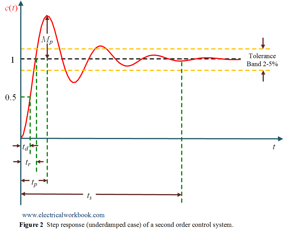
The term ${\omega _n}$ is called the natural frequency of oscillations. The term ${\omega _d} = {\omega _n}\sqrt {1 – {\xi ^2}}$ is damped frequency of oscillations. The term $\xi$ is the damping ratio and the term $\xi {\omega _n}$ is the damping factor or actual damping or damping coefficient. Also $t_d$ is delay time, $t_r$ is rise time, $t_p$ is peak time, $t_s$ is settling time and $M_p$ is peak overshoot.