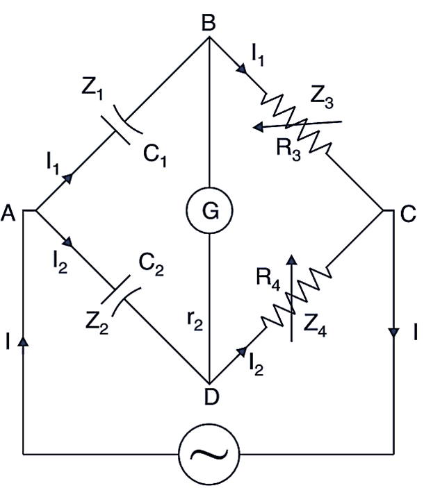
The De Sauty’s bridge is used to measure a capacitance by comparing it with another known/standard capacitance. The circuit has the following components as shown in Fig. 1.

Fig. 1: De Sauty Bridge.
C1 = unknown capacitor. whose value is to be found out.
C2 = a standard capacitor for comparison
R3, R4 = non-inductive resistors.
The balance is obtained by varying the resistor R3 (or R4).
At balance condition,
\[{{\text{Z}}_{\text{1}}}{{\text{Z}}_{\text{4}}}\text{ = }{{\text{Z}}_{\text{2}}}{{\text{Z}}_{\text{3}}}\]
\[\left( \frac{\text{1}}{\text{j}\omega {{\text{C}}_{\text{1}}}} \right)\cdot {{\text{R}}_{\text{4}}}=\left( \frac{\text{1}}{\text{j}\omega {{\text{C}}_{\text{2}}}} \right)\cdot {{\text{R}}_{\text{3}}}\]
or
\[\frac{{{\text{R}}_{\text{4}}}}{\text{j}\omega {{\text{C}}_{\text{1}}}}=\frac{{{\text{R}}_{\text{3}}}}{\text{j}\omega {{\text{C}}_{\text{2}}}}\]
or
\[\frac{{{\text{R}}_{\text{3}}}}{{{\text{R}}_{\text{4}}}}=\frac{\text{j}\omega {{\text{C}}_{\text{2}}}}{\text{j}\omega {{\text{C}}_{\text{1}}}}\]
or
\[\frac{{{\text{R}}_{\text{3}}}}{{{\text{R}}_{\text{4}}}}=\frac{{{\text{C}}_{\text{2}}}}{{{\text{C}}_{\text{1}}}}\]
or
\[{{\text{C}}_{\text{1}}}={{\text{C}}_{\text{2}}}\cdot \frac{{{\text{R}}_{\text{4}}}}{{{\text{R}}_{\text{3}}}}\]
Now C1 can be calculated as all other quantities are known.
Advantages of De Sauty’s Bridge
- It is very simple circuit.
- The calculations are also easy.
Disadvantages of De Sauty’s Bridge
- If both the capacitors are not free from dielectric loss then it is not possible to obtain the balance condition. This method therefore can be used only for air capacitors, which are more or less loss free.
Problems & Solutions in De Sauty’s Bridge
Problem 1: The null point In a De Sauty bridge is obtained in the following conditions. The arm AB of the bridge contains an unknown capacitor C1, the arm BC contains a resistor R3 = 1,400 Ω, the arm CD contains a R4 = 1,800 Ω and arm DA contains a capacitor C2 of 0.15 μF. Find the unknown capacitor C1.
Solution 1:
\[{{\text{C}}_{\text{1}}}={{\text{C}}_{\text{2}}}\cdot \frac{{{\text{R}}_{\text{4}}}}{{{\text{R}}_{\text{3}}}}\]
\[=\frac{0.15\times {{10}^{-6}}\times 1,800}{1,400}\]
\[=0.192\text{ }\!\!\mu\!\!\text{ F}\]
Thus,
\[{{\text{C}}_{1}}=0.192\text{ }\!\!~\!\!\text{ }\mu \text{ F}\]