What is Hay’s Bridge? Theory, Diagram & Derivation

Hay’s Bridge is also used for the measurement of inductance. It uses a standard capacitor in series with a resistance. With this bridge, an inductance having Q greater than 10 can also be measured.

The Fig. 1 shows the circuit diagram. The bridge has the following components.

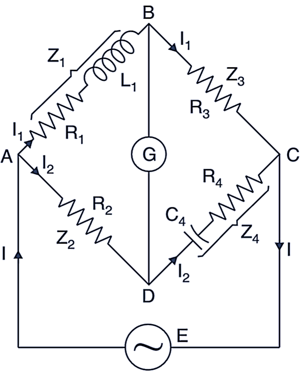
Fig. 1: Hay’s Bridge

L₁ = unknown inductance having resistance R₁

R₂, R₃, R₄ = known non-inductance resistors

C₄ = standard capacitor

At balance condition:

\[{{\text{Z}}_{\text{1}}}{{\text{Z}}_{\text{4}}}\text{ = }{{\text{Z}}_{\text{2}}}{{\text{Z}}_{\text{3}}}\]

or

\[\left[ {{\text{R}}_{\text{1}}}\text{+ j}\omega {{\text{L}}_{\text{1}}} \right]\left[ {{\text{R}}_{\text{4}}}+\frac{1}{\text{j}\omega {{\text{C}}_{\text{4}}}} \right]\text{ = }{{\text{R}}_{\text{2}}}{{\text{R}}_{\text{3}}}…(1)\]

since

\[\frac{1}{\text{j}\omega {{\text{C}}_{\text{4}}}}\text{ = }~\text{ }\!\!~\!\!\text{ }\frac{-\text{j}}{\omega {{\text{C}}_{\text{4}}}}\]

Equation 1 written as

\[\left[ {{\text{R}}_{\text{1}}}\text{+ j}\omega {{\text{L}}_{\text{1}}} \right]\left[ {{\text{R}}_{\text{4}}}-\frac{\text{j}}{\omega {{\text{C}}_{\text{4}}}} \right]\text{ = }{{\text{R}}_{\text{2}}}{{\text{R}}_{\text{3}}}\]

or

\[{{\text{R}}_{\text{1}}}{{\text{R}}_{\text{4}}}-\frac{\text{j}{{\text{R}}_{\text{1}}}}{\omega {{\text{C}}_{\text{4}}}}+{{\text{R}}_{\text{4}}}\text{j}\omega {{\text{L}}_{\text{1}}}-\frac{{{\text{j}}^{2}}\omega {{\text{L}}_{\text{1}}}}{\omega {{\text{C}}_{\text{4}}}}={{\text{R}}_{\text{2}}}{{\text{R}}_{\text{3}}}\]

or

\[{{\text{R}}_{\text{1}}}{{\text{R}}_{\text{4}}}-\frac{\text{j}{{\text{R}}_{\text{1}}}}{\omega {{\text{C}}_{\text{4}}}}+{{\text{R}}_{\text{4}}}\text{j}\omega {{\text{L}}_{\text{1}}}+\frac{{{\text{L}}_{\text{1}}}}{{{\text{C}}_{\text{4}}}}={{\text{R}}_{\text{2}}}{{\text{R}}_{\text{3}}}\]

Now equating real terms

\[{{\text{R}}_{\text{1}}}{{\text{R}}_{\text{4}}}+\frac{{{\text{L}}_{\text{1}}}}{{{\text{C}}_{\text{4}}}}={{\text{R}}_{\text{2}}}{{\text{R}}_{\text{3}}}…(2)\]

Equating imaginary terms

\[-\frac{\text{j}{{\text{R}}_{\text{1}}}}{\omega {{\text{C}}_{\text{4}}}}=-\text{j}\omega {{\text{L}}_{\text{1}}}{{\text{R}}_{\text{4}}}…(3)\]

or

\[{{\text{L}}_{\text{1}}}=\frac{{{\text{R}}_{\text{1}}}}{{{\omega }^{2}}{{\text{R}}_{\text{4}}}{{\text{C}}_{\text{4}}}}\]

Solving Equations (2) and (3), we get,

\[{{\text{R}}_{\text{1}}}=\frac{{{\omega }^{2}}{{\text{R}}_{\text{2}}}{{\text{R}}_{3}}{{\text{R}}_{\text{4}}}\text{C}_{4}^{2}}{1+{{\omega }^{2}}\text{C}_{4}^{2}\text{R}_{4}^{2}}\]

\[{{\text{L}}_{\text{1}}}=\frac{{{\text{R}}_{\text{2}}}{{\text{R}}_{3}}{{\text{C}}_{\text{4}}}}{1+{{\omega }^{2}}\text{C}_{4}^{2}\text{R}_{4}^{2}}\]

Advantages of Hay’s Bridge

1. The bridge gives very simple expression for inductance for high Q and is suitable for coils having Q more than 10.
2. This bridge requires a very low value series resistor.

Disadvantage of Hay’s Bridge

1. The Hay’s bridge is suited for coils having Q more than 10.