What is Schering Bridge? Theory, Diagram & Derivation

Schering Bridge is the most popularly used bridge for measurement of unknown capacitance and dielectric loss occurring in the capacitor. The circuit diagram of the Schering bridge is shown in Fig. 1.

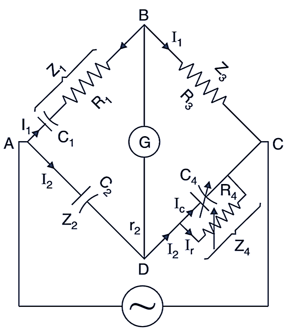
Fig. 1: Schering Bridge.

The components of the circuit are:

C₁ = The unknown capacitor

R₁ = A series resistance representing dielectric loss in the capacitor C₁

Recall that power loss in an ideal capacitor is zero. This is the resistance contained in the capacitor, which causes power loss called dielectric loss.

R_3 = a non-inductive resistor

R_4 = a variable non-inductive resistor

C₂ = a standard capacitor, is an air capacitor and is loss free

C₄ = a variable capacitor parallel with R₄

The balance is obtained by varying R₃ (or R₄).

At balance condition:

\[{{\text{Z}}_{\text{1}}}{{\text{Z}}_{\text{4}}}\text{ = }{{\text{Z}}_{\text{2}}}{{\text{Z}}_{\text{3}}}\]

or

\[\left[ {{\text{R}}_{\text{1}}}\text{+ }\frac{1}{\text{j}\omega {{\text{C}}_{\text{1}}}} \right]\left[ \frac{{{\text{R}}_{\text{4}}}}{\text{1+j}\omega {{\text{C}}_{\text{4}}}{{\text{R}}_{\text{4}}}} \right]\text{ = }\!\!~\!\!\text{  }\left[ \frac{1}{\text{j}\omega {{\text{C}}_{\text{2}}}} \right]{{\text{R}}_{\text{3}}}\]

or

\[\left[ {{\text{R}}_{\text{1}}}\text{+ }\frac{1}{\text{j}\omega {{\text{C}}_{\text{1}}}} \right]{{\text{R}}_{\text{4}}}\text{ = }\!\!~\!\!\text{  }\frac{{{\text{R}}_{\text{3}}}}{\text{j}\omega {{\text{C}}_{\text{2}}}}\left( \text{1+j}\omega {{\text{C}}_{\text{4}}}{{\text{R}}_{\text{4}}} \right)\]

or

\[{{\text{R}}_{\text{1}}}{{\text{R}}_{\text{4}}}\text{+ }\frac{1}{\text{j}\omega {{\text{C}}_{\text{1}}}}{{\text{R}}_{\text{4}}}\text{ = }\!\!~\!\!\text{  }\frac{{{\text{R}}_{\text{3}}}}{\text{j}\omega {{\text{C}}_{\text{2}}}}\text{+}\frac{\text{j}\omega {{\text{C}}_{\text{4}}}{{\text{R}}_{\text{4}}}{{\text{R}}_{\text{3}}}}{\text{j}\omega {{\text{C}}_{\text{2}}}}..(1)\]

Since,

\[\left( \frac{\text{1}}{\text{j}}=-\text{j} \right)\]

Thus, Equation 1 written as

\[{{\text{R}}_{\text{1}}}{{\text{R}}_{\text{4}}}-\frac{\text{j}{{\text{R}}_{\text{4}}}}{\omega {{\text{C}}_{\text{1}}}}=-\frac{\text{j}{{\text{R}}_{\text{3}}}}{\text{j}\omega {{\text{C}}_{\text{2}}}}\text{+}\frac{{{\text{C}}_{\text{4}}}{{\text{R}}_{\text{4}}}{{\text{R}}_{\text{3}}}}{{{\text{C}}_{\text{2}}}}\]

Now equating real terms

\[{{\text{R}}_{\text{1}}}{{\text{R}}_{\text{4}}}=\frac{{{\text{C}}_{\text{4}}}{{\text{R}}_{\text{4}}}{{\text{R}}_{\text{3}}}}{{{\text{C}}_{\text{2}}}}\]

or

\[{{\text{R}}_{\text{1}}}=\frac{{{\text{R}}_{\text{3}}}{{\text{C}}_{\text{4}}}}{{{\text{C}}_{\text{2}}}}\]

Equating imaginary terms

\[-\frac{\text{j}{{\text{R}}_{\text{4}}}}{\omega {{\text{C}}_{\text{1}}}}=-\frac{\text{j}{{\text{R}}_{\text{3}}}}{\omega {{\text{C}}_{\text{2}}}}\]

or

\[{{\text{C}}_{\text{1}}}=\frac{{{\text{R}}_{\text{4}}}{{\text{C}}_{\text{2}}}}{{{\text{R}}_{\text{3}}}}\]

Note:

(a) The schering bridge is particularly suitable for low capacitance measurement but time bridge is usually supplied from a high frequency/high voltage source.

(b) Thus bridge is like Wein bridge. The difference is that here is a R₁C₁ series circuit while in Wein bridge we use an R₁L₁ series circuit.