After reading this topic Armature controlled DC Servomotor in the control system, you will understand the theory, derivation, expressions, transfer function, and Block diagram.
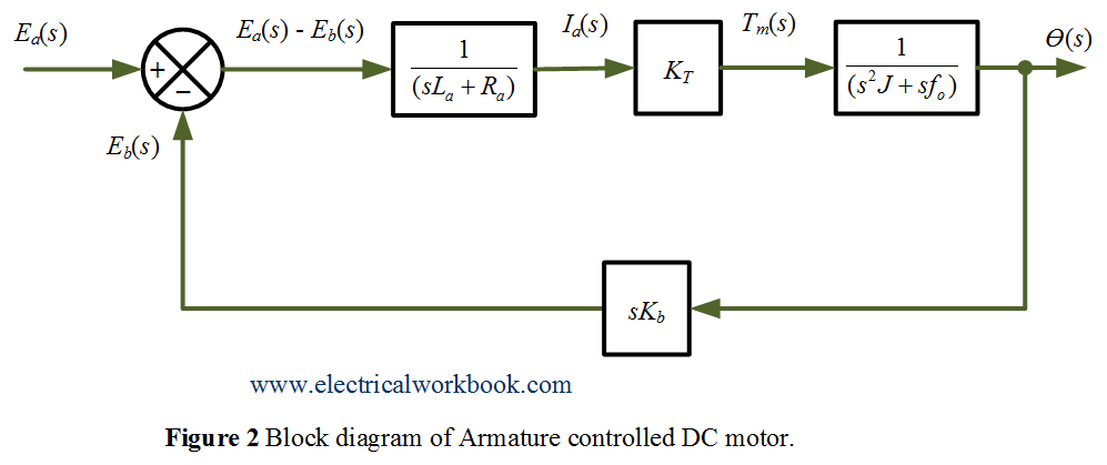
Let us consider the Armature controlled DC servomotor as shown in Figure 1.
The parameters are taken as
${R_a}$ = Armature winding resistance.
${L_a}$ = Armature winding inductance.
${i_a}$ = Armature current.
${i_f}$ = Field current.
${e_a}$ = applied armature (control) voltage.
${e_b}$ = Motor back emf.
${T_m}$ = torque developed by motor.
$\theta $ = Angular displacement of motor shaft.
$J$ = Equivalent moment of inertia of load and motor referred to motor shaft.
$f_o$ = Equivalent viscous friction coefficient of motor and load referred to motor shaft.
In armature controlled DC motors, the armature input volatge ${e_a}$ controls the motor shaft output while the field current ${i_f}$ remains constant. The DC motor operates in linear region for servo motor application. Hence, the air-gap flux $\phi $ is proportional of the field current $i_f$ as
\[\phi \propto {i_f}\]
\[\phi = {K_f}{i_f}\]
The torque $T_m$ developed by the motor is proportional to the product of armature current and air gap flux i.e.
\[{T_m} \propto \phi {i_a}\]
Also,
\[{T_m} \propto {K_f}{i_f}{i_a}\]
\[{T_m} = ({K_1}{K_f}{i_f}){i_a}\]
In armature controlled DC motors, the field current $i_f$ remains constant. Therefore,
\[{T_m} = {K_T}{i_a}\]
where, $K_T$ is the motor torque constant.
The motor back emf being proportional to speed is given by
\[{e_b} = {K_b}\left( {\frac{{d\theta }}{{dt}}} \right)….(1)\]
where, $K_b$ is the back emf constant.
Using KVL on armature circuit shown in Figure 1, the differential equation of the armature circuit is
\[{L_a}\left( {\frac{{d{i_a}}}{{dt}}} \right) + {R_a}{i_a} + {e_b} = {e_a}…(2)\]
The torque equation is
\[J\left( {\frac{{{d^2}\theta }}{{d{t^2}}}} \right) + {f_o}\left( {\frac{{d\theta }}{{dt}}} \right) = {T_m} = {K_T}{I_a}….(3)\]
Transfer function calculation of the system
Taking the Laplace transforms of Equations 1, 2 and 3 with assuming zero initial conditions, we get
\[{E_b} = s{K_b}\theta (s)…(4)\]
\[(s{L_a} + {R_a}){I_a}(s) = {E_a}(s) – {E_b}(s)…(5)\]
\[({s^2}J + s{f_o})\theta (s) = {T_m}(s) = {K_T}{I_a}(s)….(6)\]
The transfer function of the system is obtained From Equations 4, 5 and 6 as,
\[G(s) = \frac{{\theta (s)}}{{{E_a}(s)}}\]
or
\[G(s) = \frac{{{K_T}}}{{s[(s{L_a} + {R_a})(sJ + {f_o}) + {K_T}{K_b}]}}….(7)\]
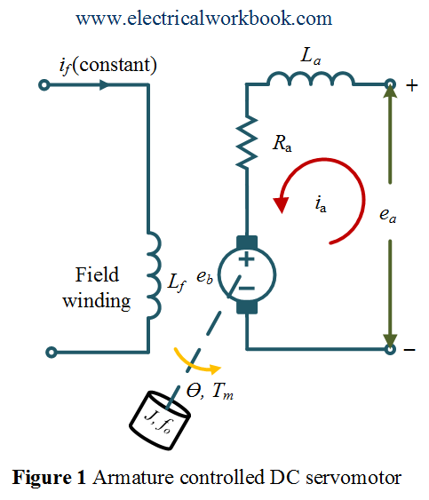
Block diagram of the system
The complete block diagram is obtained From Equations 4, 5 and 6 as shown below in Figure 2.