In this topic, you study the theory, derivation & solved examples for the Step response of the Linear Time-Invariant (LTI) System.
When the system is linear as well as time-invariant, then it is called a linear time-invariant (LTI) system.
Consider an LTI system with impulse response $h(t)$ whose input and output are $x(t)$ and $y(t)$ respectively, shown in Figure 1.
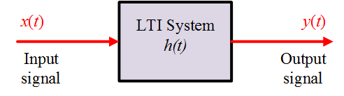
Figure 1: LTI system
When the input to LTI system is unit impulse $\delta (t)$ then the output of LTI system is known as impulse response $h(t)$. Mathematically,
\[y(t) = x(t) * h(t)\]
Similarly, for the input to LTI system is unit step signal $ u(t)$ then the output of LTI system is known as step response $s(t)$. Mathematically,
\[s(t) = h(t) * u(t)\]
Using convolution property of thr Laplace transform,
\[S(s) = H(s) \cdot \frac{1}{s}\]
Also,
\[H(s) = s \cdot S(s)\]
Applying inverse laplace transform,
\[h(t) = \frac{d}{{dt}}s(t)\]
And
\[s(t) = \int\limits_{ – \infty }^t {h(\tau )d\tau } \]
Example : The unit impulse response of a system is $h(t) = – 4{e^{ – t}} + 6{e^{ – 2t}}$. What will be the step response of the same system for $t$ ≥ $0$.
Solution: Impulse response $h(t) = – 4{e^{ – t}} + 6{e^{ – 2t}}$
Step response is given by
\[s(t) = \int\limits_{ – \infty }^t {h(t)dt } \]
\[s(t) = \int\limits_{ – \infty }^t {( – 4{e^{ – t}} + 6{e^{ – 2t}})dt} \]
\[s(t) = {4{e^{ – t}} – 3{e^{ – 2t}}} {\text{ + constant}} \]