After reading this y parameter in two port network, you will understand the theory, how to determine y parameters, the condition of symmetry & reciprocity and applications.
General theory of y parameters
In two port network, the terminal input and output voltages V1 and V2 can be expressed in terms of the terminal input and output currents I1 and I2.
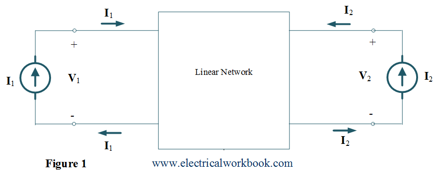
As shown in Figure 1, the terminal voltages can be written in terms of the terminal currents as
${{\mathbf{I}}_1} = {{\mathbf{y}}_{{\text{11}}}}{{\mathbf{V}}_1} + {{\mathbf{y}}_{{\text{12}}}}{{\mathbf{V}}_2}$ ….(1)
${{\mathbf{I}}_2} = {{\mathbf{y}}_{{\text{21}}}}{{\mathbf{V}}_1} + {{\mathbf{y}}_{{\text{22}}}}{{\mathbf{V}}_2}$ ….(2)
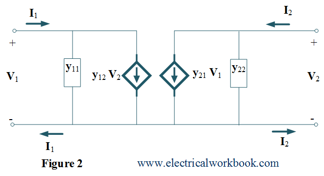
From Eq.(1) and Eq.(2), it can be concluded that the terminal currents are dependent variables and the terminal voltages are independent variables. Also, using the Eq.(1) and Eq.(2), the equivalent circuit represented as shown in Figure 2.
 By using Eq.(1) and Eq.(2), can be written in matrix form as
$\left[ {\begin{array}{*{20}{c}}
{{{\mathbf{I}}_1}} \\
{{{\mathbf{I}}_2}}
\end{array}} \right] = \left[ {\begin{array}{*{20}{c}}
{{{\mathbf{y}}_{{\text{11}}}}}&{{{\mathbf{y}}_{{\text{12}}}}} \\
{{{\mathbf{y}}_{{\text{21}}}}}&{{{\mathbf{y}}_{{\text{22}}}}}
\end{array}} \right]\left[ {\begin{array}{*{20}{c}}
{{{\mathbf{V}}_1}} \\
{{{\mathbf{V}}_2}}
\end{array}} \right]$
The above matrix can be generalized as
$\left[ {\mathbf{I}} \right] = \left[ {\mathbf{y}} \right]\left[ {\mathbf{V}} \right]$
where [y] matrix,
$\left[ {\mathbf{y}} \right] = \left[ {\begin{array}{*{20}{c}}
{{{\mathbf{y}}_{{\text{11}}}}}&{{{\mathbf{y}}_{{\text{12}}}}} \\
{{{\mathbf{y}}_{{\text{21}}}}}&{{{\mathbf{y}}_{{\text{22}}}}}
\end{array}} \right]$
The elements of matrix [y] are called y parameters and each parameters having unit in mho.
How to determine y parameters?
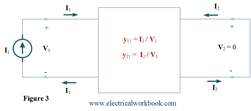
- The y parameters y11 and y21 are obtained by short circuiting the port 2 i.e. V2 = 0 along with connecting current source I1 to port 1 as shown in Figure 3. Thus we get
\[{{\mathbf{y}}_{{\text{11}}}} = {\left. {\frac{{{{\mathbf{I}}_1}}}{{{{\mathbf{V}}_1}}}} \right|_{{{\mathbf{V}}_2} = 0}}\]
${{\mathbf{y}}_{{\text{11}}}}{\text{is Short – circuit driving point input admittance}}{\text{.}}$
\[{{\mathbf{y}}_{{\text{21}}}} = {\left. {\frac{{{{\mathbf{I}}_2}}}{{{{\mathbf{V}}_1}}}} \right|_{{{\mathbf{V}}_2} = 0}}\]
${{\mathbf{y}}_{{\text{21}}}}{\text{ is Short – circuit forward transfer admittance}}{\text{.}}$
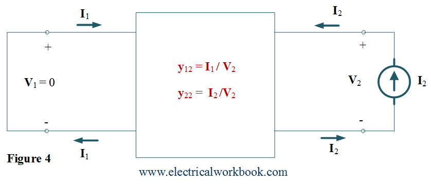
- The y parameters y22 and y12 are obtained by short circuiting the port 1 i.e. V1 = 0 along with connecting current source I2 to port 2 as shown in Figure 4. Thus we get
\[{{\mathbf{y}}_{{\text{12}}}} = {\left. {\frac{{{{\mathbf{I}}_1}}}{{{{\mathbf{V}}_2}}}} \right|_{{{\mathbf{V}}_1} = 0}}\]
${{\mathbf{y}}_{{\text{12}}}}{\text{ is Short – circuit reverse transfer admittance}}{\text{.}}$
\[{{\mathbf{y}}_{22}} = {\left. {\frac{{{{\mathbf{I}}_2}}}{{{{\mathbf{V}}_2}}}} \right|_{{{\mathbf{V}}_1} = 0}}\]
${{\mathbf{y}}_{22}}{\text{ is Short – circuit driving point output admittance}}{\text{.}}$
Note:- For y parameters, the terminal currents I1 and I2 are function of terminal voltages V1 and V2 as
$\left( {{{\mathbf{I}}_1},{{\mathbf{I}}_2}} \right) = {\text{f }}\left( {{{\mathbf{V}}_1},{{\mathbf{V}}_2}} \right)$
Condition of symmetry
A two port network is said to be symmetrical if the ratio of response to excitation remains same at both ports independently with respect to the defined circuit conditions such as open circuit or short circuit. Thus, we can say
\[{\left. {\frac{{{{\mathbf{I}}_1}}}{{{{\mathbf{V}}_1}}}} \right|_{{{\mathbf{V}}_1} = 0}} = {\left. {\frac{{{{\mathbf{I}}_2}}}{{{{\mathbf{V}}_2}}}} \right|_{{{\mathbf{V}}_2} = 0}}\]
\[{\text{or, }}{{\mathbf{y}}_{11}} = {{\mathbf{y}}_{22}}\]
Condition of reciprocity
A two port network is said to be reciprocal if the ratio of response to excitation remains same even when the position of response to excitation are interchanged. Thus, we can say
\[{\left. {\frac{{{{\mathbf{I}}_1}}}{{{{\mathbf{V}}_2}}}} \right|_{{{\mathbf{V}}_1} = 0}} = {\left. {\frac{{{{\mathbf{I}}_2}}}{{{{\mathbf{V}}_1}}}} \right|_{{{\mathbf{V}}_2} = 0}}\]
\[{\text{or, }}{{\mathbf{y}}_{12}} = {{\mathbf{y}}_{21}}\]
Applications
- Use for filters Combination.
- design of impedance-matching networks
- design of power distribution networks.