MATLAB Ordinary differential equations

After reading the MATLAB Ordinary differential equations topic, you will able to implement and solve differential equations in MATLAB.

An ODE is a differential equation with an independent variable, a dependent variable, and having some initial value for each variable.

Steps for solving a differential equation using MATLAB

• Create a function or an anonymous function for the given problem.
• Select ODE solver
• Use ODE command to solve ODE.

Note:- See on the MATLAB contents, for creating a function or anonymous function.

ODE solver

MATLAB provides various inbuilt ODE solvers as shown below to solve ODE.

Solver	Description	Method
ode45	Nonstiff differential equations	Runge-Kutta
ode23	Nonstiff differential equations	Runge-Kutta
ode113	Nonstiff differential equations	Adams
ode15s	Stiff differential equations	NDFs
ode23s	Stiff differential equations	Rosenbrocks
ode23t	Moderately stiff differential equations	Trapezoidal rule
ode23tb	Stiff differential equations	TR-BDFs

ODE command

ODE command is used to solve an initial value ODE problem. The general form is:

[t,y] = ODE_name(ODEfun,tspan,y0)

where,

• ODE_name Is the name of the solver (numerical method).
• ODEfun is the name of an anonymous function.
• tspan is the interval of the solution.
• y0 is the initial value of y.

Example

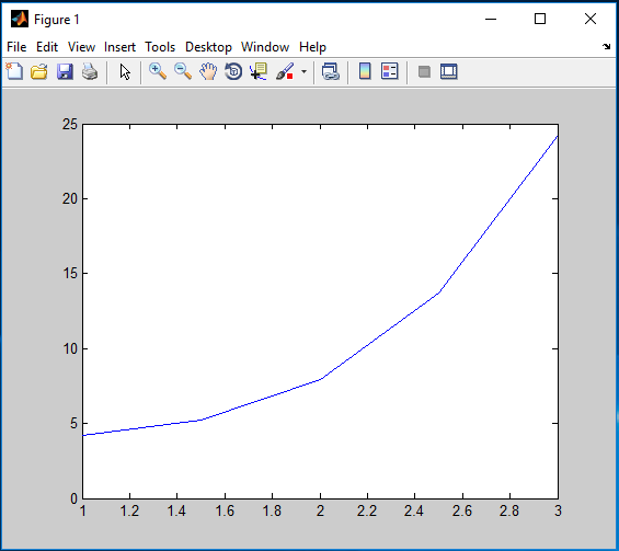
Aim (1): To solve differential equation given below, using MATLAB.

$\frac{{dy}}{{dt}} ={t^3}$

for 1 ≤ t ≤ 3 with y = 4.2  at t = 1

Program (1):

% defining anonymous function

ode1=@(t,y)(t^3)


[t y]=ode45(ode1,[1:0.5:3],4.2);

plot(t,y)

Output (1):

ode1 =

@(t,y)(t^3)