After reading the MATLAB Polynomials topic, you will able to solve problems based on polynomials in MATLAB, you will also understand how to create polynomials, evaluating polynomials, find polynomials roots, find derivative of polynomials, etc.
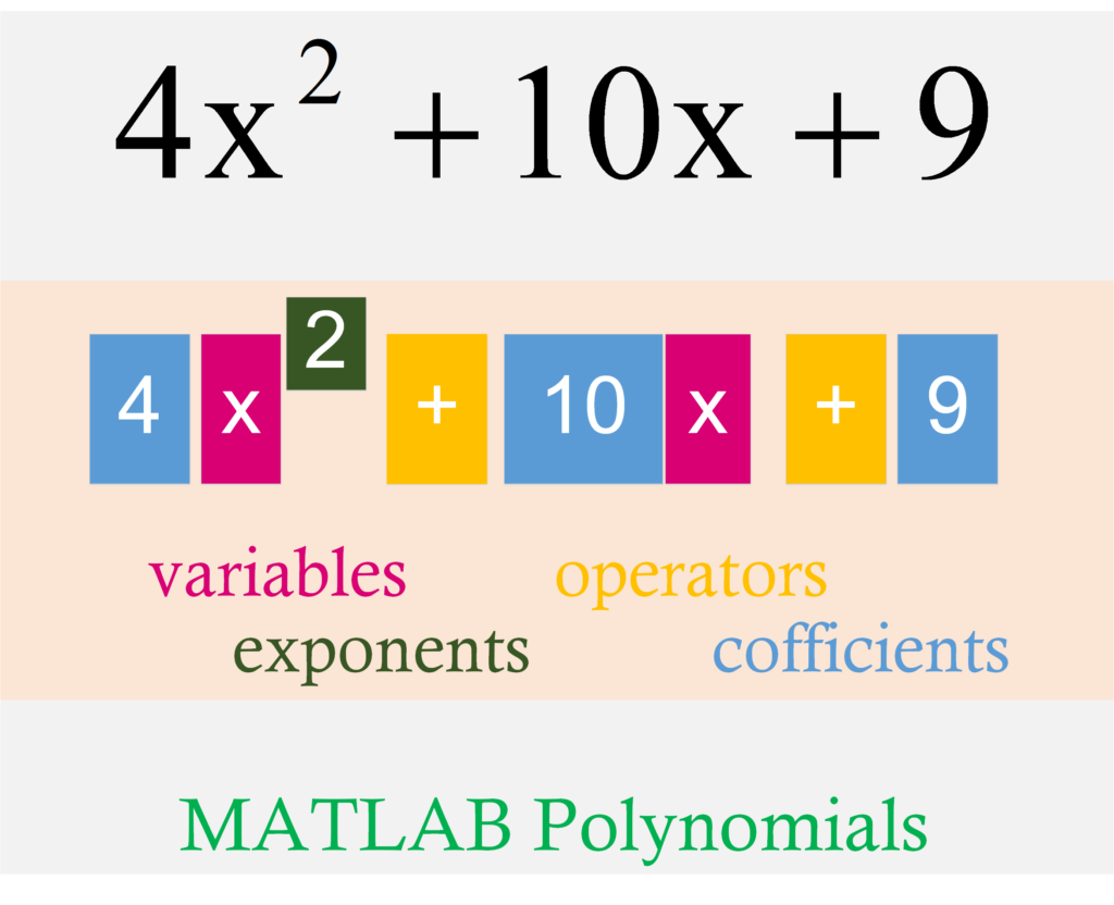
In MATLAB, polynomials are represented as row vectors having coefficients ordered by descending powers.
Example
Aim (1): To represent polynomial equation p(x) as given below, in MATLAB.
\[p(x) = {x^3} – 4x + 10\]
Program (1):
p=[1 0 -4 10]
Output (1):
p = 1 0 -4 10
Polynomial Evaluation
The value of a polynomial at a specified point. The general form of polynomial evaluation is
General Form:
polyval(p,5)
where,
- p is a row vector with the coefficients of the polynomial.
- p is evaluated at a specific value 5.
Example
Aim (1): To evaluate polynomial equation p(x) as given below at x = 5 , in MATLAB.
\[p(x) = {x^3} – 4x + 10\]
Program (1):
p=[1 0 -4 10];
polyval(p,5)
Output (1):
ans = 115
Polynomial Roots
The roots are the values for which the polynomial value results to zero. The general form of polynomial evaluation is
General Form:
r=roots(p)
where,
- r is a column vector with the roots of the polynomial.
- p is a row vector with the coefficients of the polynomial.
Example
Aim (1): To find roots of polynomial equation p(x) as given below, in MATLAB.
\[p(x) = {x^3} – 4x + 10\]
Program (1):
p=[1 0 -4 10];

r=roots(p)
Output (1):
r =
  -2.7608 + 0.0000i
   1.3804 + 1.3102i
   1.3804 - 1.3102i
Polynomial Derivatives
The polyder function used to calculate the derivative of any polynomial.
General Form:
d=polyder(p)
where,
- d is a row vector with the roots of the polynomial derivatives.
- p is a row vector with the coefficients of the polynomial.
Example
Aim (1): To find derivative of polynomial equation p(x) as given below, in MATLAB.
\[p(x) = {x^3} – 4x + 10\]
Program (1):
p=[1 0 -4 10];

d=polyder(p)
Output (1):
d =

     3     0    -4
\[d(x) = 3{x^2} – 4\]
Polynomials Multiplication (Convolution)
The polynomials multiplication is done by using convolution operation. The MATLAB built-in conv function is used to perform the convolution operation
Example
Aim (1): To multiply two polynomials p(x) and q(x) as given below, in MATLAB.
\[p(x) = {x^2} – 2x + 10\]
\[q(x) = 2{x^2} + 4x + 7\]
Program (1):
p=[2 -2 10];

q=[2 4 7];

c=conv(p,q)
Output (1):
c =

     4     4    26    26    70
\[c(x) = 4{x^4} + 4{x^3} + 26{x^2} + 26x + 70\]
Polynomials Division (Deconvolution)
The polynomials division is done by using deconvolution operation. The MATLAB built-in deconv function is used to perform the deconvolution operation
Example
Aim (1): To divide two polynomials p(x) and q(x) as given below, in MATLAB.
\[p(x) = 3{x^2} – 2x + 4\]
\[q(x) = {x^2} + 7\]
Program (1):
p=[2 9 7 -6];

q=[1 3];

[a,b]=deconv(p,q)
Output (1):
a =

     2     3    -2

b =

     0     0     0     0
\[a(x) = 2{x^2} + 3x – 2\]
and remainder is zero as
\[b(x) = 0\]
Polynomials Curve Fitting
The polynomials curve fitting is the process that fits a set of data to a polynomial. The general form of polynomial curve fitting command is
General Form:
p=polyfit(x,y,n)
where,
- x is a vector with the x-axis coordinates of the data points.
- y is a vector with the y-axis coordinates of the data points.
- n is the degree of the polynomial.
Example
Aim (1): To demonstrate curve fitting in MATLAB.
Program (1):
% create x vector

x=[1 2 3 4 5];

% create y vector

y=[2.3 4 5.67 23.4 345];

%consider third degree polynomial, n=3

p=polyfit(x,y,3)
Output (1):
p =

   25.3250 -181.0779  387.0671 -232.8960
\[p(x) = 25.325{x^3} – 181.0779{x^2} + 387.0671x – 232.896\]