After reading this Nodal Analysis topic of electric or network circuits, you will understand the theory and also able to apply it in numerical problems.
In the nodal analysis, we need to calculate node voltages so that circuit branch current can find out easily.
Procedure for applying Nodal Analysis: –
- Identify the total number of nodes.
- One node selected as the reference node, also it is assigned to have a ground (zero) potential and the remaining nodes called as nonreference node and we assign voltage designations to nonreference nodes.
- Develop the KCL equations for each nonreference node.
- Solve the equations to find the unknown node voltages.
Note:-
- The total number of equations (e) required to solve the network with the help of nodal analysis is
e = N – 1.
where N is the total number of nodes.
- Nodal analysis is applicable for both planar and nonplanar network.
Examples
Example 1. For the given network, find current I using Nodal analysis.
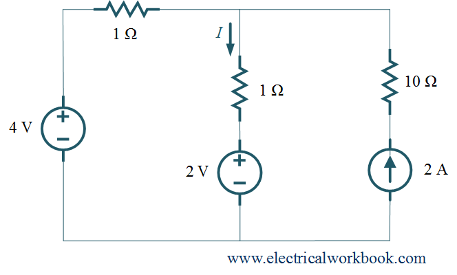
Solution: Let’s follow the Procedure for applying Nodal Analysis
Step 1: – The total number of nodes is 2.
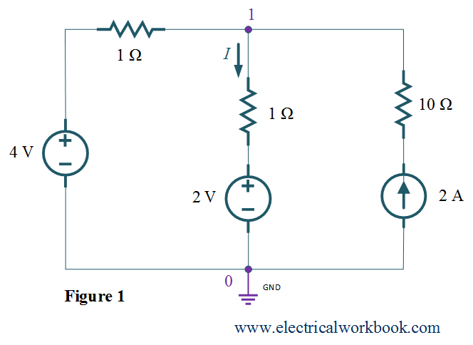
Step 2: – Node 0 is selected as reference node and it is assigned to have ground (zero) potential and the remaining node 1 as non-reference node as shown in Figure 1.
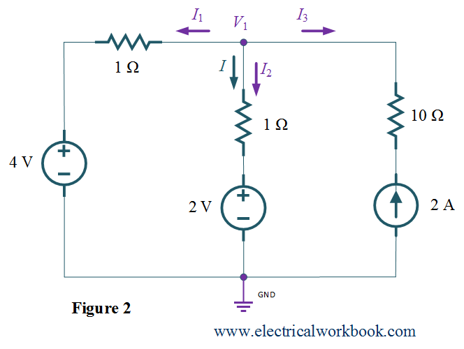
Step 3 and Step 4: – Apply KCL to node 1 as shown in Figure 2, gives
\[{I_1} + {I_2} + {I_3} = 0\]
\[\frac{{({V_1} – 0) – 4}}{1} + \frac{{({V_1} – 0) – 2}}{1} + ( – 2) = 0\]
${V_1} = 4{\text{V}}$
\[{\text{also, }}I = {I_2}\]
\[{I_2} = \frac{{({V_1} – 0) – 2}}{1} = \frac{{(4 – 0) – 2}}{1} = 2\]
Thus,
\[I = 2{\text{ A}}{\text{.}}\]
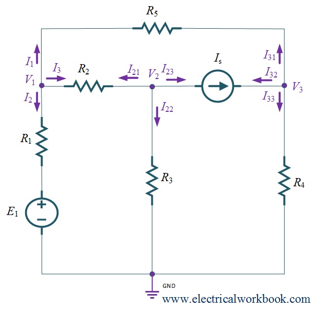
Example 2. For the given network, write the Nodal equations.
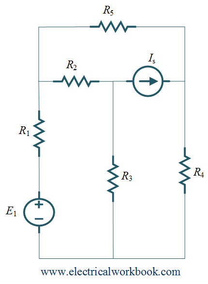
Solution: Let’s follow the Procedure for applying Nodal Analysis
Step 1: – The total number of nodes is 4.
Step 2: – Node 0 is selected as reference node and it is assigned to have ground (zero) potential and the remaining nodes 1, 2 and 3 as non-reference node as shown in Figure 1.
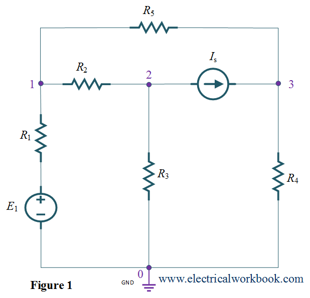
Step 3: – Apply KCL to node 1, 2 and 3 as shown in Figure 2,
KCL at node 1 gives,
\[{I_1} + {I_2} + {I_3} = 0\]
\[\frac{{{V_1} – {V_3}}}{{{R_5}}} + \frac{{\left( {{V_1} – 0} \right) – E}}{{{R_1}}} + \frac{{{V_1} – {V_2}}}{{{R_2}}} = 0\]
KCL at node 2 gives,
\[{I_{21}} + {I_{22}} + {I_{23}} = 0\]
\[\frac{{{V_2} – {V_1}}}{{{R_2}}} + \frac{{{V_2} – 0}}{{{R_3}}} + {I_S} = 0{\text{ }}({\text{as }}{I_{23}} = {I_S})\]
KCL at node 3 gives,
\[{I_{31}} + {I_{32}} + {I_{33}} = 0\]
\[\frac{{{V_3} – {V_1}}}{{{R_5}}} – {I_S} + \frac{{{V_3} – 0}}{{{R_4}}} = 0{\text{ }}({\text{as }}{I_{32}} = – {I_S})\]