What is Dual Cycle? Process, Derivation, Diagram & Efficiency

Dual combustion cycle is a combination of constant pressure and constant volume cycle where, heat is added partly at constant volume and remaining at constant pressure. This cycle is also called mixed cycle or limited pressure cycle. This cycle is represented on P-V and T-s diagram as given below,

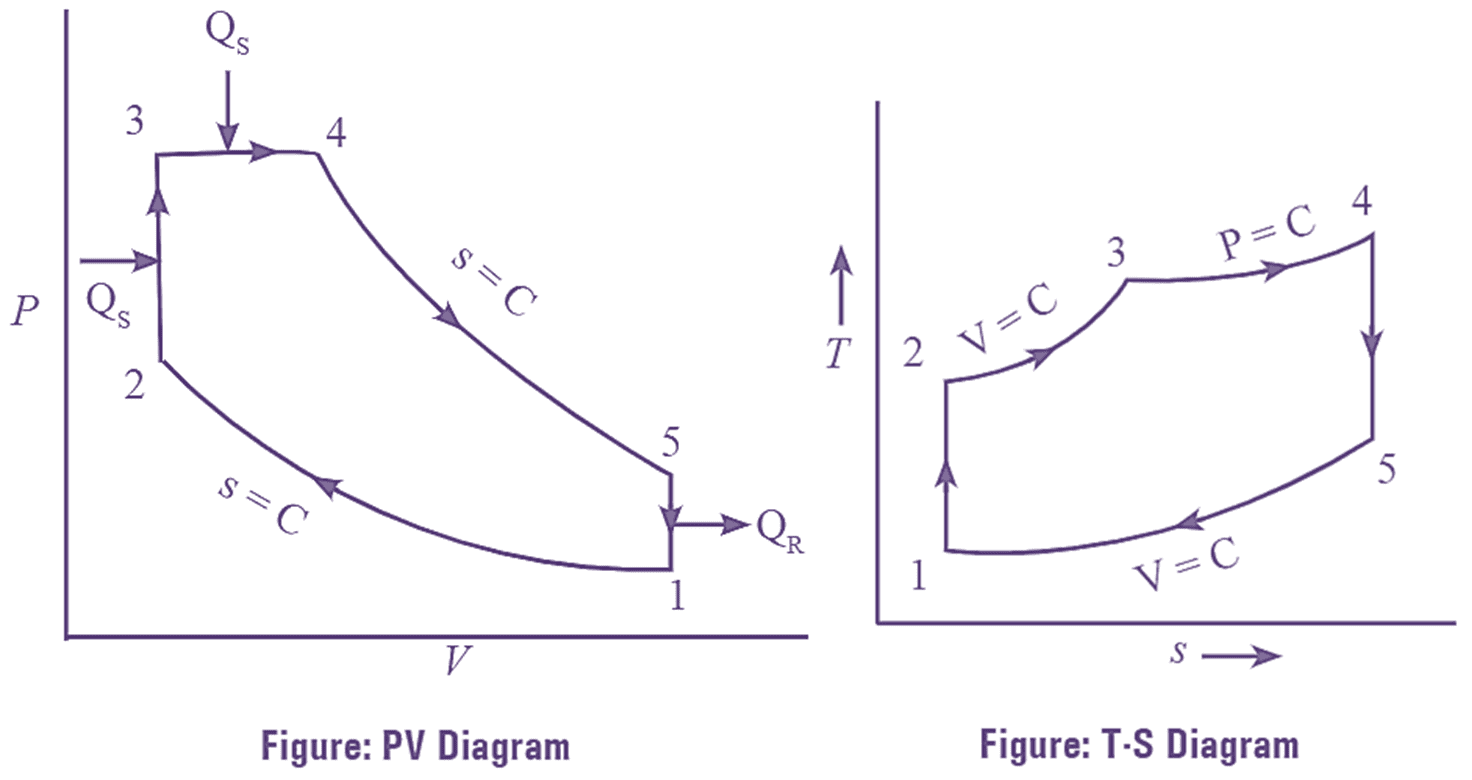
Figure 1: Dual Cycle.

Dual combustion cycle consists of five processes. They are.

Process 1-2: Isentropic compression – It is a reversible adiabatic compression process during which pressure and temperature increases from P₁, T₁ to P₂, T₂ respectively.

Process 2-3: Reversible constant volume heat addition – During this process, heat is added to the air at constant volume by a suitable heating source such that the pressure and temperature increases from P₂, T₂, to P₃, T₃ respectively.

Process 3-4: Reversible constant pressure heat addition – During this process, heat is added at constant pressure by a suitable heating source such that the volume and temperature increases from V₃, T₃ to V₄, T₄  respectively.

Process 4-5: Isentropic expansion – It is a reversible adiabatic expansion process during which the pressure and temperature decreases from P₄ ,T₄ to P₅, T₅ respectively.

Process 5-1: Reversible constant volume heat rejection – During this process. heat is rejected at constant volume such that the pressure and temperature falls from P₅, T₅ to P₁, T₁ respectively.

Heat supplied,

Q₁ = mC_v (T₃ – T₂) + mC_p (T₄ – T₃)

Heat rejected,

Q₂ = mC_v (T₅ – T₁)

Work done =   Heat supplied  ˗ Heat rejected

\[W={{Q}_{1}}-{{Q}_{2}}\]

\[=m{{C}_{v}}({{T}_{3}}-{{T}_{2}})+m{{C}_{p}}({{T}_{4}}-{{T}_{3}})-m{{C}_{v}}({{T}_{5}}-{{T}_{1}})\]

Thermal efficiency

\[\eta =\frac{Work\text{ }done}{Heat\text{ }added}\]

\[=\frac{m{{C}_{v}}({{T}_{3}}-{{T}_{2}})+m{{C}_{p}}({{T}_{4}}-{{T}_{3}})-m{{C}_{v}}({{T}_{5}}-{{T}_{1}})}{m{{C}_{v}}({{T}_{3}}-{{T}_{2}})+m{{C}_{p}}({{T}_{4}}-{{T}_{3}})}\]

\[=1-\frac{m{{C}_{v}}({{T}_{5}}-{{T}_{1}})}{m{{C}_{v}}({{T}_{3}}-{{T}_{2}})+m{{C}_{p}}({{T}_{4}}-{{T}_{3}})}\]

Therefore,

\[ \eta =1-\frac{{{T}_{5}}-{{T}_{1}}}{({{T}_{3}}-{{T}_{2}})+({{T}_{4}}-{{T}_{3}})}\]

\[\text{  }\gamma =\frac{{{C}_{p}}}{{{C}_{v}}}\]

Now,

Compression ratio,

\[r=\frac{{{V}_{1}}}{{{V}_{2}}}\]

Expansion ratio,

\[{{r}_{e}}=\frac{{{V}_{5}}}{{{V}_{4}}}\]

Cut-off ratio,

\[\rho =\frac{{{V}_{4}}}{{{V}_{3}}}\]

Pressure ratio,

\[{{r}_{p}}=\frac{{{P}_{3}}}{{{P}_{2}}}\]

Consider process 1-2,

\[\frac{{{T}_{2}}}{{{T}_{1}}}={{\left( \frac{{{V}_{1}}}{{{V}_{2}}} \right)}^{\gamma -1}}={{\left( r \right)}^{\gamma -1}}\]

\[{{T}_{2}}={{T}_{1}}\text{  }{{\text{r}}^{\gamma -1}}\]

Consider process 2-3,

\[\frac{{{T}_{3}}}{{{T}_{2}}}=\frac{{{P}_{3}}}{{{P}_{2}}}={{r}_{p}}\]

\[{{T}_{3}}={{T}_{2}}\text{ }{{r}_{p}}={{T}_{1.}}\text{ }{{\text{r}}^{\gamma -1}}.{{r}_{p}}.\rho \]

Consider process 3-4,

\[\frac{{{V}_{4}}}{{{T}_{4}}}=\frac{{{V}_{3}}}{{{T}_{3}}}\]

\[{{T}_{4}}=\frac{{{V}_{4}}}{{{V}_{3}}}{{T}_{3}}\]

\[=\rho {{T}_{3}}={{T}_{1.}}\text{ }{{\text{r}}^{\gamma -1}}{{r}_{p}}.\rho \]

Consider process 4-5,

\[\frac{{{T}_{5}}}{{{T}_{4}}}={{\left( \frac{{{V}_{4}}}{{{V}_{5}}} \right)}^{\gamma -1}}={{\left( \frac{{{V}_{4}}}{{{V}_{1}}} \right)}^{\gamma -1}}\]

\[={{\left[ \frac{{{V}_{4}}}{{{V}_{3}}}\times \frac{{{V}_{3}}}{{{V}_{2}}}\times \frac{{{V}_{2}}}{{{V}_{1}}} \right]}^{\gamma -1}}\]

\[{{V}_{3}}={{V}_{2}}\]

\[={{\left[ \frac{{{V}_{4}}}{{{V}_{3}}}\times \frac{{{V}_{2}}}{{{V}_{1}}} \right]}^{\gamma -1}}\text{ }\]

\[={{\left( \frac{\rho }{r} \right)}^{\gamma -1}}\]

\[{{T}_{5}}={{T}_{4}}.{{\left( \frac{\rho }{r} \right)}^{\gamma -1}}\]

\[={{T}_{1}}{{r}^{\gamma -1}}.{{r}_{p}}.\rho .{{\left( \frac{\rho }{r} \right)}^{\gamma -1}}\]

\[={{T}_{1}}{{r}_{p}}.{{\rho }^{\gamma }}\]

Substitute eq.(2)(3)(4)and(5)in eq.(1),

Then,

\[\eta =1-\frac{{{T}_{1}}\left( {{r}_{p}}{{\rho }^{\gamma }}-1 \right)}{{{T}_{1}}\left( {{r}^{\gamma -1}}{{r}_{p}}-{{r}^{\gamma -1}} \right)+\gamma {{T}_{1}}\left( {{r}^{\gamma -1}}{{r}_{p}}\rho -{{r}^{\gamma -1}}{{r}_{p}} \right)}\]

\[=1-\frac{\left( {{r}_{p}}{{\rho }^{\gamma }}-1 \right)}{{{r}^{\gamma -1}}\left( {{r}_{p}}-1 \right)+\gamma .{{r}^{\gamma -1}}{{r}_{p}}\left( \rho -1 \right)}\]

\[=1-\frac{\left( {{r}_{p}}{{\rho }^{\gamma }}-1 \right)}{{{r}^{\gamma -1}}\left[ \left( {{r}_{p}}-1 \right)+\gamma .{{r}_{p}}\left( \rho -1 \right) \right]}\]

\[=1-\frac{1}{{{r}^{\gamma -1}}}\left[ \frac{\left( {{r}_{p}}{{\rho }^{\gamma }}-1 \right)}{\left[ \left( {{r}_{p}}-1 \right)+\gamma .{{r}_{p}}\left( \rho -1 \right) \right]} \right]\]

The efficiency of dual cycle is function r, ρ, r_p and γ.