An equation relating the relative motion of the rotor axis with respect to stator field in time domain is known as swing equation.
or
The equation which describes the behavior of a synchronous machine during transient period is known as swing equation.
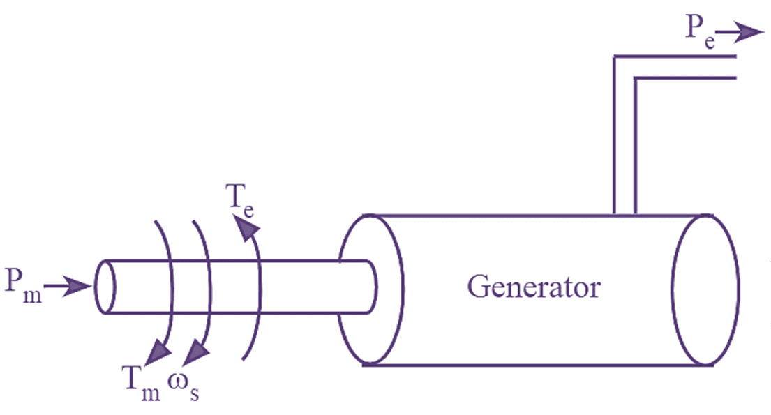
Figure 1.
Derivation of Swing Equation
Consider the synchronous machines showing the flow of mechanical and electrical power as shown in figure (1)
Let,
θ – Angular displacement in radians
ω – Angular velocity in radian/sec
α – Angular acceleration in radians/sec2
Tm – Turbine torque in N-m
Te – Electromagnetic torque in N-m
J – Moment of inertia in kg-m2.
When the synchronous machine is acting as a generator (see Figure 1), Tm is the input and Te is the output and in case of generator, the accelerating torque is given by,
\[{{T}_{a}}={{T}_{m}}-{{T}_{e}}…(1)\]
Multiplying equation (1) with ‘ω’, we get,
\[\omega {{T}_{a}}=\omega {{T}_{m}}-\omega {{T}_{e}}\]
Since,
\[P=\omega T\]
\[{{P}_{a}}={{P}_{m}}-{{P}_{e}}…(2)\]
Where,
Pa = Accelerating power
Pm = Mechanical power
Pe = Electrical power.
We know that,
\[{{T}_{a}}=J\alpha \]
\[{{P}_{a}}=J\alpha \omega \]
\[=\left( J\omega \right)\alpha \]
But,
\[M=J\omega \]
\[{{P}_{a}}=M\alpha …(3)\]
Where, M is the angular momentum.
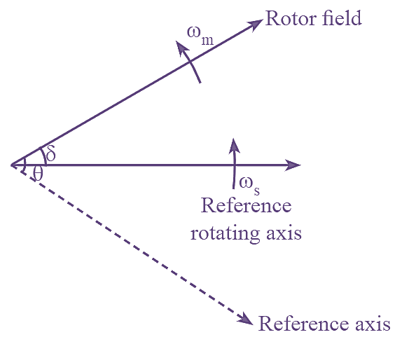
Figure 2
The variation of angular position and velocity with respect to synchronously rotating axis is shown in figure (2). From figure (2),
\[\theta ={{\omega }_{s}}t+\delta …(4)\]
Where, δ = Load angle (or) Torque angle
Differentiating equation (4) with respect to t, we get,
\[\frac{d\theta }{dt}={{\omega }_{s}}+\frac{d\delta }{dt}\]
Again differentiating above equation with respect to t,
\[\frac{{{d}^{2}}\theta }{d{{t}^{2}}}=\frac{{{d}^{2}}\delta }{d{{t}^{2}}}\]
But,
\[\frac{{{d}^{2}}\theta }{d{{t}^{2}}}=\alpha \]
Thus
\[\alpha =\frac{{{d}^{2}}\delta }{d{{t}^{2}}}…(5)\]
From equation (3),
\[{{P}_{a}}=M\alpha \]
\[\alpha =\frac{{{P}_{a}}}{M}…(6)\]
Using equation (2), in equation (6), we get,
\[\alpha =\frac{{{P}_{m}}-{{P}_{e}}}{M}…(7)\]
Substituting equation (5) in equation (7), we get,
\[\frac{{{d}^{2}}\delta }{d{{t}^{2}}}=\frac{{{P}_{m}}-{{P}_{e}}}{M}\]
\[M\frac{{{d}^{2}}\delta }{d{{t}^{2}}}={{P}_{m}}-{{P}_{e}}…(8)\]
or
\[\frac{H}{\pi f}\frac{{{d}^{2}}\delta }{d{{t}^{2}}}={{P}_{m}}-{{P}_{e}}\]
Equation (8) is called the swing equation. It explains the rotor dynamics for a synchronous machine. It also describes the behavior of a synchronous machine during transient period.
Swing equation is a second order non-linear differential equation since the electrical power, Pe = Pmax sin δ is based on the sine of angle δ.
The swing equation is given by,
\[M\frac{{{d}^{2}}\delta }{d{{t}^{2}}}={{P}_{m}}-{{P}_{e}}\]
Or
\[\frac{H}{\pi f}\frac{{{d}^{2}}\delta }{d{{t}^{2}}}={{P}_{m}}-{{P}_{e}}\]
Where,
M = Inertia constant in p.u
H = Inertia constant in NIJ/MVA
f = Frequency in Hz
δ = Power angle in electrical radians
Pm = Mechanical power input in p.u
Pe = Electrical power output in p.u.
Swing Curve
Swing Curve Swing curve is a graph drawn between the torque angle (δ) on Y-axis and time (t) on X-axis. It is generally drawn for a transient state to study the nature of variations in torque angle (δ) for sudden disturbances. The variation of ‘δ’ with respect to time ‘t’ is shown in figure 3,
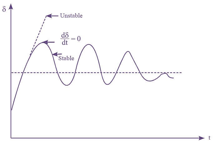
Figure 3: Swing Curve.
Swing curve explains the behavior of a synchronous machine during transient and gives information regarding the stability of a power system for any disturbance. These curves are very useful in determining the effectiveness of relay protection on power system with respect to the fault clearance before one or more machines become unstable and lose synchronism.
Importance of Swing Equation
In power system, the swing equation has a great importance for the study of transient stability. The swing equation is used to determine the stability of a rotating synchronous machine within a power system. When swing equation is solved, the expression for ‘δ’ is obtained, which the function of time. The graph of this solution is known as ‘Swing Curve’ of the machine. By investigating the swing curves of overall machines connected to the system we can know whether the machines continue in synchronous or not after a disturbance. The following graph represents the variations in δ with respect to time t. From the above graph the condition $\frac{d\delta }{dt}=0$ indicates that the system is stable and if, $\frac{d\delta }{dt}>0$, then the system is unstable.