What is RL Series Circuit? Circuit Diagram, Phasor Diagram, Derivation & Formula

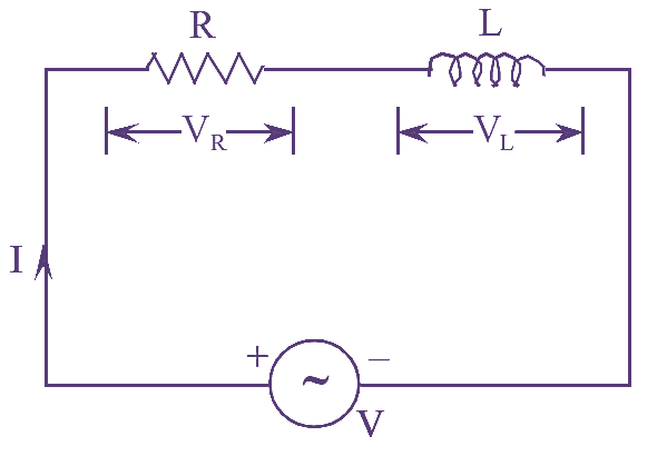
Figure (1): RL Series Circuit.

An RL series circuit consisting of a resistor of ‘R’ Ohm in series with an inductance of ‘L’ Henrys connected to an A.C supply as shown in figure (l).

Applying Kirchhoff’s voltage law to the circuit shown in figure (1), we get,

\[V={{V}_{R}}+{{V}_{L}}\]

Where,

V = Source voltage

V_R = Voltage drop across resistor = IR

V_L = Voltage drop across inductor IX_L

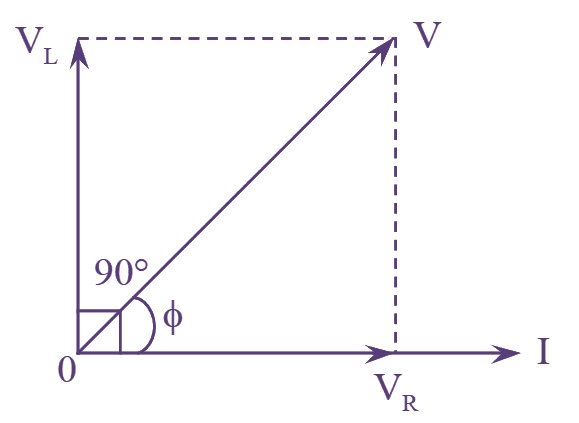
Figure (2): RL Series Circuit Phasor Diagram.

The phasor diagram is drawn by taking the current ‘I’ as reference phasor as shown in figure (2).

The voltage drop ‘V_R‘ is in phase with current I since R is a pure resistance and voltage drop ‘V_L‘ leads current ‘I’ by 90º since L is a pure inductance.

From the phasor diagram, we have,

\[{{V}^{2}}=V_{R}^{2}+V_{L}^{2}\]

\[=\sqrt{V_{R}^{2}+V_{L}^{2}}\]

\[=\sqrt{{{\left( IR \right)}^{2}}+{{\left( I{{X}_{L}} \right)}^{2}}}=I\sqrt{R_{{}}^{2}+X_{L}^{2}}\]

\[V=IZ\]

Where, Z = Impedance in ohms $=\sqrt{R_{{}}^{2}+X_{L}^{2}}$

Figure (3): RL Series Circuit Impedance Triangle.

The phase difference angle $\phi$ can be determined from impedance triangle as shown in figure (3).

\[\tan \phi =\frac{AB}{OA}\]

\[\tan \phi =\frac{{{X}_{L}}}{R}\]

\[\phi ={{\tan }^{-1}}\frac{{{X}_{L}}}{R}\]

The power factor of the circuit is given by $\cos \phi$, since it is the cosine function of the phase angle between voltage and current.

\[\cos \phi =\frac{R}{Z}\]

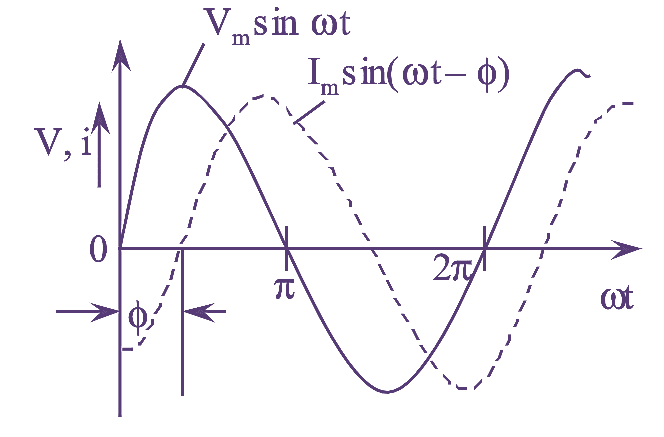
Figure (1): RL Series Circuit Waveforms.

Let applied voltage, v = V_m sinωt

Then, equation of current will be,

\[i={{I}_{m}}\sin \left( \omega t-\phi  \right)\]

\[P=vi\]

\[=\left( {{V}_{m}}\sin \omega t \right)\left( {{I}_{m}}\sin \left( \omega t-\phi  \right) \right)\]

\[=\frac{1}{2}{{V}_{m}}{{I}_{m}}\left[ 2\sin \omega t\sin \left( \omega t-\phi  \right) \right]\]

\[=\frac{{{V}_{m}}{{I}_{m}}}{2}\left[ \cos \phi -\cos \left( 2\omega t-\phi  \right) \right]\]

\[=\frac{{{V}_{m}}{{I}_{m}}}{2}\cos \phi -\frac{{{V}_{m}}{{I}_{m}}}{2}\cos \left( 2\omega t-\phi  \right)\]

In the above expression the first term $\frac{{{V}_{m}}{{I}_{m}}}{2}\cos \phi $ represents the steady power, since V_m, I_m and are fixed in magnitude. The second term $\frac{{{V}_{m}}{{I}_{m}}}{2}\cos \left( 2\omega t-\phi  \right)$ represents the fluctuating power, which is zero over one full cycle.

The average power (or) total power,

\[P=\frac{{{V}_{m}}{{I}_{m}}}{2}\cos \phi\]

\[=\left( \frac{{{V}_{m}}}{\sqrt{2}} \right)\left( \frac{{{I}_{m}}}{\sqrt{2}} \right)\cos \phi \]

\[=VI\cos \phi \]

Where, V and I are r.m.s values of voltage and current.